How-To: Carry UAVs through Indian airport security in 2022

TL:DR - Pack the UAVs in check-in luggage. Pack the controllers + batteries in cabin baggage. Empty out the contents of the cabin baggage into the tray while passing through security.

Note: This is a brief post describing our learnings regarding the transport of UAVs through Indian airport security in 2022. It is written in the hope that it helps other Indian UAV users navigate airport security without delay. I don’t think this will apply to non-Indian UAV operators, especially if they don’t present as Indian.

At Technology for Wildlife Foundation, one of our core operations is the use of robots (both Unmanned Aerial Vehicles and Unmanned Underwater vehicles) for conservation data acquisition purposes. For some projects, our partners send us data they’ve collected using their own devices. However, for others, it is imperative that we be on site with our equipment. This occasionally necessitates the transport of our robots across the country. For sites close to our base in Goa, India, we travel by either road or by rail. For these modes of transport, our primary concern is to package the equipment securely to avoid damage during transit. While traveling by air, however, we need to put much more thought into transporting our equipment.

As of November 2021, UAV users in India have a clear set of guidelines to follow, in the form of the Drone Rules 2021. As UAVs have become more mainstream, the security establishment is also formalising and mainstreaming processes around UAVs. To transport drones within the country, the Central Industrial Security Force (CISF), who manage security at most of India’s airports, now seem to have guidelines on how to process UAVs at domestic airport security checkpoints.  

Based on whether baggage is being carried in the cargo hold or in the passenger cabin, there are two categories of baggage on flights: cabin, which accompanies the passenger, and check-in, which goes into the hold. In brief, drone batteries and controllers (which contain fixed batteries) must be carried in the passenger cabin, while the drones themselves (without any batteries) must be carried in the cargo hold. If the controller batteries are removable, the controllers can also go into check-in baggage, which may be required depending on the size and weight of the controller. UAVs with fixed batteries cannot be carried on domestic airlines.

Pack the drones carefully, in a locked piece of luggage, as they will be out of sight passing through the luggage handling process, which can be rough on fragile items. The check-in luggage is deposited at the counter. In the past, with other robotic devices, we have informed the check-in staff that there are complex devices within the luggage. I personally have been called to check-in luggage security to verify what exactly the device is. Informing the check-in staff that the luggage contains UAVs without batteries is not required by regulations. While it may be helpful, it may also invite additional unnecessary scrutiny and is not something that we have felt the need to do regularly.

When going through security with our cabin baggage, we place every single piece of electronic equipment into the security tray that passes through the conveyor belt. When security staff have enquired as to the purpose of the devices, a straightforward answer of either “batteries”, or “drone batteries and controllers, but the drones have been checked-in”, has sufficed so far. We also carry paperwork that describes how the drones are to be used and have been used in the past; for us specifically, these consist of permission letters from the Forest Department.  

At some point in late 2021 or early 2022, posters depicting what cannot be carried as cabin baggage have been expanded to include drones as an additional item at the bottom of the poster. We’ll update this post with a photo of the poster the next time we have the opportunity. In the meanwhile, do let us know about your own experiences transporting UAVs by air in the comment section.

Tracking Air Pollution

As winter commences in North India, the presence of PM2.5 makes it to the headlines in New Delhi. Particulate matter, (PM) in particular PM2.5 is the classification of fine inhalable particles, with diameters that are generally 2.5 micrometers and smaller. In comparison, human hair ranges from 50-70 micrometers which makes the fine particulate matter, PM2.5 in this case, 30 times smaller in size and hence inhalable. Health and visibility problems are caused in New Delhi post-monsoon due to the burning of paddy in the states of Punjab and Haryana, India. The paddy is harvested during the month of October and wheat is sown swiftly after. The management of paddy stubble in the time interval between harvest and sowing of wheat is crucial. 

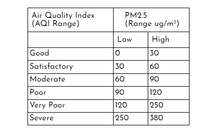
The wind carries the residue of the burnt paddy (PM2.5) through to Delhi and the city consequently experiences ‘very poor’ to ‘severe’ air quality levels during the winter months. The acceptable limits based on the health impacts of PM2.5 are shown in Table 1.

Table 1: AQI Range of PM2.5

We created spatial data visualisations highlighting the deteriorating air quality in Northern India due to the burning of paddy, to accompany an article in Mongabay-India. The Mongabay article gives an insight into what stops the paddy from turning into biofuel - covering the technical, financial and official handicaps. A part of the article explored the mapping of paddy burning locations from September to November, 2021 and the PM2.5 mapping from October to November, 2021. 

In this post, we share how satellite imagery of PM2.5 was processed and animated to display the severity of air pollution by using ECMWF’s CAMS Global Near Real Time data from Google Earth Engine (GEE) data catalogue. The time period of 1st October, 2021 to 30th November, 2021 was chosen to highlight the PM2.5 levels post harvest-season.

First, a Daily-Means algorithm is prepared to aggregate data so that one day in the said time-interval has one output image of PM2.5. In this case, mean is used to aggregate the daily data into one image. At the end of this step, we have an Image Collection of 61 daily images with PM2.5 for each day (Figure 1).

Figure 1: Daily Mean algorithm

This image collection is then clipped to the desired extent (using the in-built clip function of GEE). The Daily-Means image collection data can also be added to the GEE map display panel using the Map.addLayer function. In this case, the mean function was used to display the Image Collection output in the Layers Panel.

Figure 2: Image Collection display

The next step is to create the animated dataset using the image collection. In this case, a scale bar, title and outline of state boundaries (Punjab and Haryana, India) of the image are displayed in the final animation. The scale bar is positioned by specifying its coordinates. Its maxima and minima labels, that is the PM2.5 levels as well as its style: font-size, colour, etc, can also be customised. At the same time, the title and its style are chosen and rendered. The outline of the required area which is captured in the animation is added next. The scale bar, title and outline are then blended into the Daily Means map using the in-built blend function of GEE. Next, the overall coverage of the extent of the animation is specified with coordinates-this extent subsumes the scale, title, outline and other add-ons of the animation around the actual map of interest. The visualization parameters of the animated dataset are then specified and printed to the console (Figure 3). The styling of animation felt a bit tedious as the arrangement of add-ons (scale bar, tittle, etc) is relative to the latitude longitude coordinates of the map of interest. Although it makes the dataset visualisation accurate, moving the add-ons needs careful calculations.

Figure 3: Animation display

The following animation (Figure 4) was used to visualize the impact of burning paddy in Punjab, Haryana and New Delhi, india.

Figure 4: Animated PM2.5

Although the intensity of pollution seems linked to the increase in the number of burning locations, there were some glitches in interpreting the scale of the data provided. Scale of the data varies from 0 to 0.1 ug/m3 according to the dataset provider’s unit during the said time-period for the concerned area shown in Figure 4. The actual scenario of PM2.5 levels in the air is evidently greater than the permissible limits. While we share the process of animating the PM2.5 data, we are trying to better understand its scale as well. 

It took around two days to piece the code together. While this was sufficient, a host of other options are available at ‘users/gena/packages’ (Figure 5) in the Script Manager section of the GEE code editor interface which can be harnessed to load more information on the animated dataframes based on the requirement. I hope to further explore this package for better application and visualization.

Figure 5: Package for animation

The animated dataset here shows us the change in air quality. While this gives us a peep into reality, we hope to see all paddy turn into biofuel soon. If you have any questions or comments, get in touch with us at contact@techforwildlife.com.

Using Computer Vision to Identify Mangrove-containing pixels in Satellite Imagery

This blogpost has been written by a team of 3rd-year BTech students from PES College, Bangalore: B Akhil, Mohammad Ashiq, Hammad Faizan and Prerana Ramachandra . They are collaborating with us on a research project around the use of computer vision and satellite imagery for mangrove conservation purposes.

Mangroves are plants  that grow in salt marshes, muddy coasts and tidal estuaries. They are biodiversity hotspots and serve as nurseries for fish stocks. They also help in maintaining the quality of water by filtering out the pollutants and sediments. Mangroves can flourish  in places where no other tree can grow, which makes them important ecosystems that help prevent coastal erosion and provide protection from flooding and cyclonic events. Furthermore, mangroves have the highest per-unit area rates of carbon sequestration (Alongi 2012) among any ecosystem, terrestrial or marine. Despite the ecosystem services they provide, mangrove forests are among the most threatened ecosystems on the planet. Globally, we have already lost 30-50% of all mangroves forests (WWF Intl. 2018) in the last 50 years and mangroves continue to be cut at rates 3-5 times higher than terrestrial forests every year.

One part of the solution in the puzzle to better conserve mangroves is to better document and monitor their existence, and the ecosystem services that they provide. So far, Technology for Wildlife has used traditional remote sensing methods on satellite and RPA imagery to understand the extent of mangroves. Our team is experimenting with the  use of computer vision to detect mangroves in satellite imagery. Through this project, we hope to develop this technique and compare its accuracy with that obtained using traditional spatial analysis methods. We  are also interested in this project because of the possibility of implementing a machine learning model that could become better  at detecting mangroves over time. Finally, the prospect of creating an automated monitoring system that systematically evaluates satellite data and detects changes in mangrove cover could be a significant tool for the conservation of mangrove ecosystems, both in Goa as well as globally.

In the rest of this post, we will outline the methods we considered for this project , as well as our reasoning for our final selections. The three major categories of  methods we considered for this project are:

(i)Machine Learning approaches, 

ii)Deep Learning approaches and 

iii) Image Processing Techniques. 

The Machine Learning approach  includes techniques such as decision trees, which is an approach of vegetation classification done by matching the spectral features or combinations of spectral features from images with those of possible end members of vegetation types. Other techniques include K-Means and IsoData algorithms, both of which are unsupervised, easy to apply and widely available in image processing, geospatial information and statistical software packages. 

The Deep Learning approach deals with architectures such as classification using Siamese residual networks (SiResNet) in which a 3-D Siamese residual network with a spatial pyramid pooling (3-D-SiResNet-SPP) is used which learns discriminative high-level features for hyperspectral mangrove species classification with limited training samples. Other potential techniques which could be used for better training of the model is the Chopped picture method, where images are dissected into numerous small squares so as to efficiently produce training images, and Convolutional Neural Networks, which are a class of deep neural  networks, most commonly applied to analyzing visual imagery. One could also use Mask - RCNN, which is a deep neural network designed to solve instance segmentation problems in machine learning or computer vision algorithms. An architecture which can be used for segmentation is a U-net neural network which is a standard CNN architecture for image segmentation tasks.

Under Image Processing, the techniques available include Gabor Filtering (which is widely used in image texture segmentation) feature extraction (where we use Hadooop to extract features from large datasets) and the Colour based approach (it deals with methods like k-means clustering and colour extraction using HSV model), among others. 

Choosing an appropriate method depends significantly on the data available. For training our model we have used USGS EarthExplorer to download Landsat 8 images. Each image consists of 8 channels, containing spectral information across several different wavelengths in the visible and near-infrared portions of the electromagnetic spectrum. The samples used to train the model were labeled at the pixel-level i.e. each pixel in the sample has an attribute value.  These attribute values are binary in nature, with a value of 1 representing the presence of mangroves, and a value of 0 indicating the absence of mangroves. Due to the limited spatial resolution of Landsat images, direct visual interpretation is difficult. The criteria initially used to label the mask data were a combination of altitude values from SRTM data and NDVI values from Landsat 8 data. If a specific pixel meets the required criteria to be tagged as ‘mangrove’, then it is labeled with a value of 1, or else given a value of 0.  For future iterations, we’ll be developing a masking process that includes aerial imagery and more sophisticated spatial analyses.

The method we chose for our project is segmentation using a U-net neural network. U-Net is considered to be a standard CNN architecture for image segmentation tasks. Segmentation is similar to image classification but in segmentation instead of just classifying the image based on the object present each pixel is classified to belong to a specific class i.e. segmentation requires discrimination at pixel level. U-net was originally invented and first used for biomedical image segmentation. Its architecture can be broadly thought of as an encoder network followed by a decoder network. 

The encoder is the first half of the architecture. It is usually a pre-trained classification network like VGG/ResNet where convolution blocks are applied first, followed by  maxpool downsampling to encode the input image into feature representations at multiple different levels. The decoder is the second half of the architecture. The goal here is to semantically project the discriminative features learnt by the encoder onto the pixel space to get a dense classification. The decoder consists of upsampling and concatenation followed by regular convolution operations. Upsampling is done to restore the condensed feature map to the original size of the input image, therefore expanding the feature dimensions. Upsampling is also referred to as transposed convolution, upconvolution, or deconvolution.

The U-net architecture offers some advantages over other segmentation techniques. In U-net architecture, the network is input-image size agnostic since it does not contain fully connected layers. This also leads to a smaller model weight size, hence also making it computationally efficient. The architecture is easily understandable, and can be scaled to have multiple classes. Architecture works well with a small training set, due to the robustness provided with data augmentation.

Deep U-net architecture is employed to perform segmentation. Image augmentation is used for input images to significantly increase training data. Image augmentation is also done while testing and mean results are exported.We plan on using Tensorflow Keras with python and its libraries to build our model, which we’ll be running on real-world data.

If you have any questions or comments on our work, please reach out to us through the contact form on the website.