Mudflats to Mangroves

‘Tyācī sarva khāraphuṭīcī jamīna | It's all mangroves now.’ 

Growing where land and water meet, mud collected around the tangled mangrove roots, with shallow mudflats surrounding them. Patches of mangroves alongside the river were pointed out to us by our guide, an elder from the village, with the repeated observation – ‘it’s all mangroves now’ – as we walked on the river banks of the Savitri in Maharashtra.

We conducted this field trip in May 2022, with our collaborators Farmers for Forests (F4F) and EcoNiche to test a pilot model that encourages mangrove regeneration on fallow land unsuitable for agriculture.

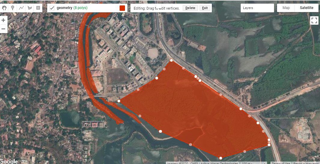
Mangrove presence in Raigad, Maharashtra

Mangroves are found in tropical and subtropical latitudes, growing in slow-moving waters that allow sediments to accumulate. All species of the mangrove plant produce fruits, seeds, and seedlings that float in the oceans before taking root in fresh, brackish water. Muck builds up around the seedling’s roots, forming the surface for mudflats. In a few years, as the trees grow, the land area surrounding them also increases, growing an ecosystem around themselves. Because of their ability to act as carbon sinks, mangroves are often acknowledged as a compelling nature-based solution (NbS) to fight climate change. In November 2021, TfW and EcoNiche pitched a project that was selected for WRI’s Land Accelerator Grant which is aimed at business programmes to restore degraded forests and farmlands. Focusing on mangrove and seagrass conservation, the project, named the Reimagining Coasts Initiative, made it to the top 3% of nearly 500 applicants and won the innovation grant. Through this grant, we explored possible mangrove conservation and plantation in rural Maharashtra with our collaborators Farmers for Forests (F4F) who work in the area, and are familiar with local stakeholders. 

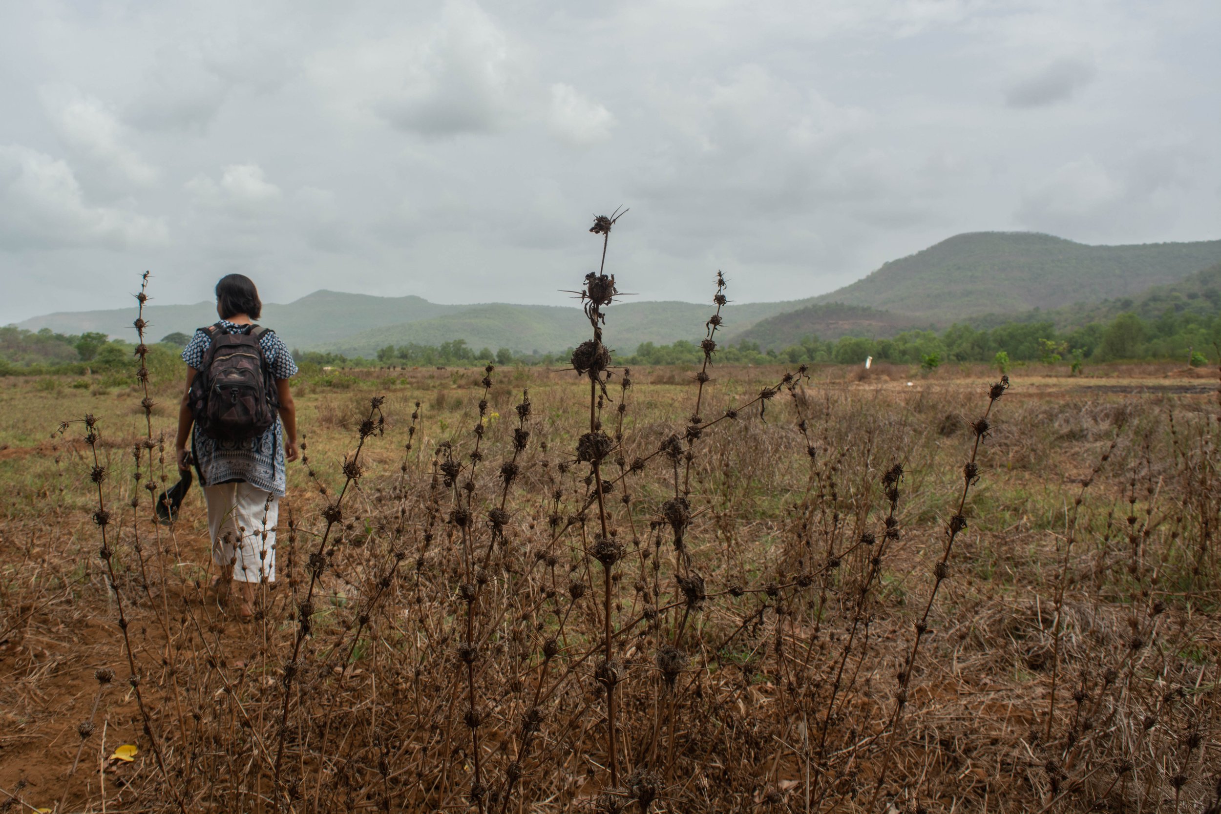
These villages on the river banks are within 30 to 50 km of the Arabian sea. Farming practices here evolved to include the raising of bunds to prevent saline backflow into the fields from the river. Community construction and maintenance of these bunds allowed agriculture to develop in the region. However, in present times, these bunds have collapsed from lack of maintenance due to the dwindling of the farming community. As per the elders of the community, a variety of factors, such as the search for a better quality of life, different career options and monetary benefit, to name a few, have led to the younger generation migrating to urban centres. At this point, the population of the village consists primarily of senior citizens. The resulting increase in salination has rendered parts of these lands unsuitable for agriculture and has seen the natural return of mangroves. This makes this an interesting site to investigate mangrove restoration and conservation.

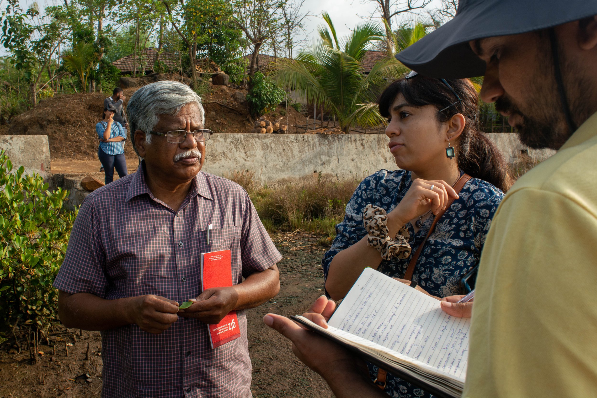
Team members interacting with an interested landowner to verify site location.

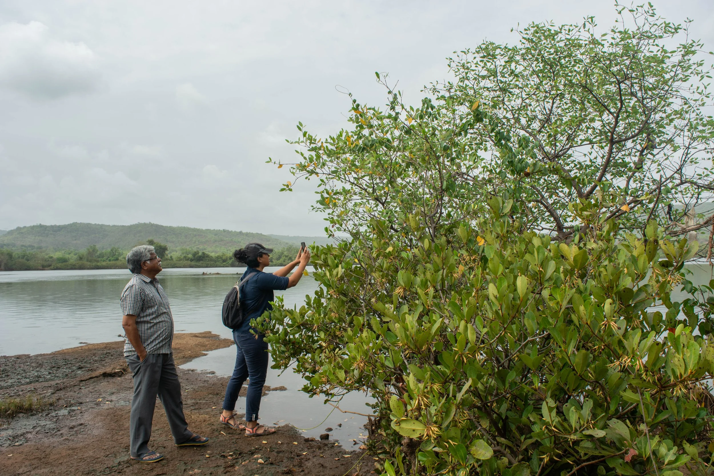
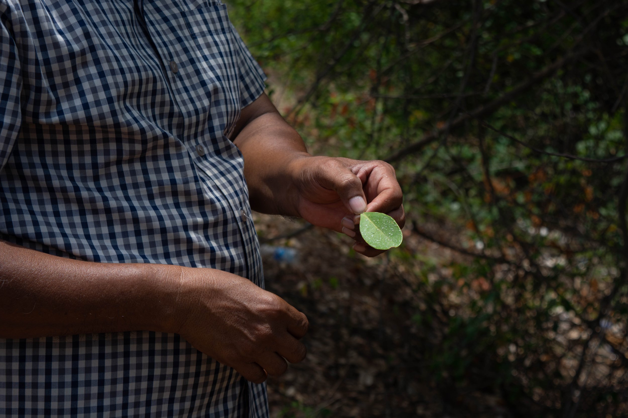
For their projects, the current model by F4F begins with the establishment of a dialogue with landowners in the region who may be interested in plantation or restoration on their land, in return for financial benefits. In this case, they were exploring restoration of mangroves, a new endeavour for them. Our field trip began with discussions with landowners and the village sarpanch, who had prior engagement with F4F. We were also joined by Dr. V. Selvam, an authority on mangroves in India. Accompanied by village elders, we walked through the village, to the edge of the river bank; to trace the path of salinity in their lands. This process helped us identify the main channels and breaks in bunds, while understanding the extent of salinity-induced features. Dr. Selvam guided us with information on the mangrove ecosystem flora while identifying the mangrove family and sub-varieties, while we took copious notes. We carried out photo-documentation of the species, while simultaneously listing their presence manually by noting scientific names, common names and local names. 

This exercise was repeated in every site we visited during this field visit. We also used our Uncrewed Aerial Vehicle (UAV) to aerially survey potential sites for mangrove restoration. The aerial imagery collected was used to discuss the land that landowners were interested in inducting into our project. This was a task that would have taken longer and been far more taxing if our surveys were restricted to the ground alone. Alternatively, using satellite or land survey based maps, the precision and understanding of the decision making may have been affected.

In the weeks following the field trip, we found that some policy blocks prevented us from seeing the project through to implementation. However, it has opened an avenue for us to explore and work towards for the future, and in other regions.

A combination of data gained from the ground, coupled with remote monitoring offers new opportunities to monitor nature-based solutions (NbS). However, standard operating procedures for carrying out such surveys, with information on the methods and tools, require further development. We are actively engaged in this journey to refine techniques for using this data– to inclusively plan and effectively monitor restoration efforts.

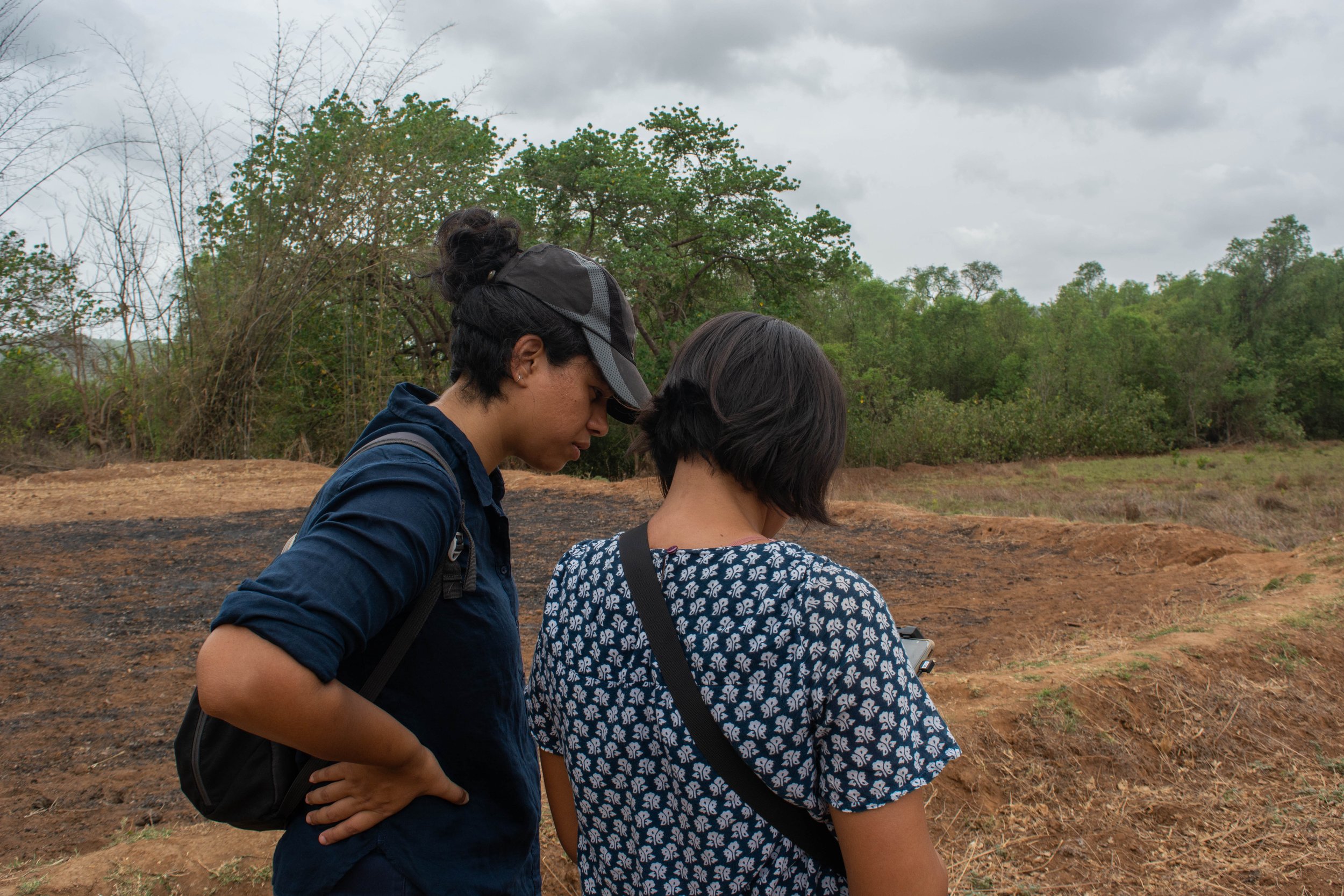
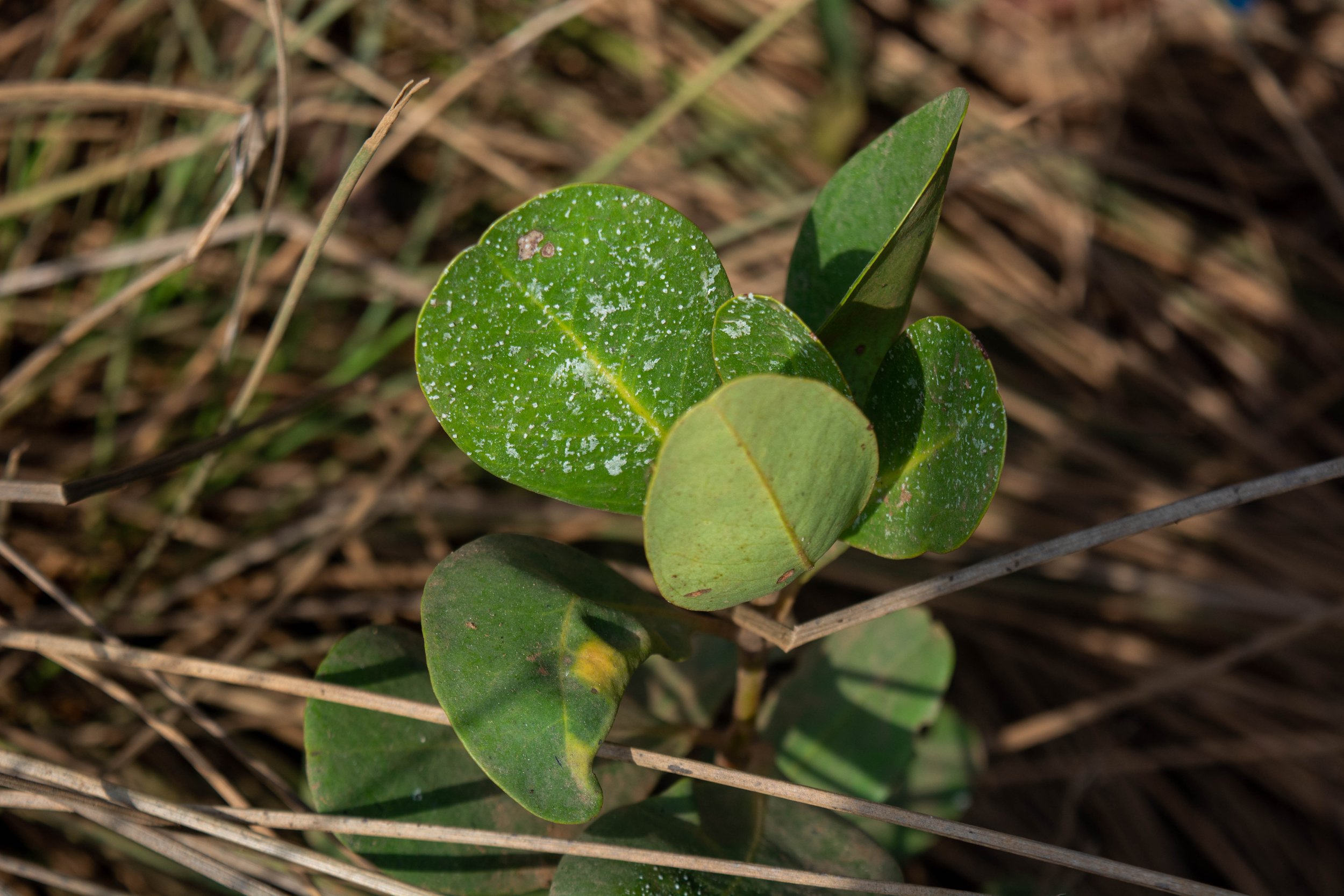
Presence of halophytic weed in a potential site for mangrove forestation.

Globally, there is a growing tendency towards ramping up the use of nature-based solutions. Enhancing ecosystems on the whole and addressing social concerns while generating environmental, economic, and societal value, NbS can help restore damaged ecosystems and carry out conservation efforts. These efforts ultimately have net positive impact, both locally and globally, benefitting the climate.

Using Computer Vision to Identify Mangrove-containing pixels in Satellite Imagery

This blogpost has been written by a team of 3rd-year BTech students from PES College, Bangalore: B Akhil, Mohammad Ashiq, Hammad Faizan and Prerana Ramachandra . They are collaborating with us on a research project around the use of computer vision and satellite imagery for mangrove conservation purposes.

Mangroves are plants  that grow in salt marshes, muddy coasts and tidal estuaries. They are biodiversity hotspots and serve as nurseries for fish stocks. They also help in maintaining the quality of water by filtering out the pollutants and sediments. Mangroves can flourish  in places where no other tree can grow, which makes them important ecosystems that help prevent coastal erosion and provide protection from flooding and cyclonic events. Furthermore, mangroves have the highest per-unit area rates of carbon sequestration (Alongi 2012) among any ecosystem, terrestrial or marine. Despite the ecosystem services they provide, mangrove forests are among the most threatened ecosystems on the planet. Globally, we have already lost 30-50% of all mangroves forests (WWF Intl. 2018) in the last 50 years and mangroves continue to be cut at rates 3-5 times higher than terrestrial forests every year.

One part of the solution in the puzzle to better conserve mangroves is to better document and monitor their existence, and the ecosystem services that they provide. So far, Technology for Wildlife has used traditional remote sensing methods on satellite and RPA imagery to understand the extent of mangroves. Our team is experimenting with the  use of computer vision to detect mangroves in satellite imagery. Through this project, we hope to develop this technique and compare its accuracy with that obtained using traditional spatial analysis methods. We  are also interested in this project because of the possibility of implementing a machine learning model that could become better  at detecting mangroves over time. Finally, the prospect of creating an automated monitoring system that systematically evaluates satellite data and detects changes in mangrove cover could be a significant tool for the conservation of mangrove ecosystems, both in Goa as well as globally.

In the rest of this post, we will outline the methods we considered for this project , as well as our reasoning for our final selections. The three major categories of  methods we considered for this project are:

(i)Machine Learning approaches, 

ii)Deep Learning approaches and 

iii) Image Processing Techniques. 

The Machine Learning approach  includes techniques such as decision trees, which is an approach of vegetation classification done by matching the spectral features or combinations of spectral features from images with those of possible end members of vegetation types. Other techniques include K-Means and IsoData algorithms, both of which are unsupervised, easy to apply and widely available in image processing, geospatial information and statistical software packages. 

The Deep Learning approach deals with architectures such as classification using Siamese residual networks (SiResNet) in which a 3-D Siamese residual network with a spatial pyramid pooling (3-D-SiResNet-SPP) is used which learns discriminative high-level features for hyperspectral mangrove species classification with limited training samples. Other potential techniques which could be used for better training of the model is the Chopped picture method, where images are dissected into numerous small squares so as to efficiently produce training images, and Convolutional Neural Networks, which are a class of deep neural  networks, most commonly applied to analyzing visual imagery. One could also use Mask - RCNN, which is a deep neural network designed to solve instance segmentation problems in machine learning or computer vision algorithms. An architecture which can be used for segmentation is a U-net neural network which is a standard CNN architecture for image segmentation tasks.

Under Image Processing, the techniques available include Gabor Filtering (which is widely used in image texture segmentation) feature extraction (where we use Hadooop to extract features from large datasets) and the Colour based approach (it deals with methods like k-means clustering and colour extraction using HSV model), among others. 

Choosing an appropriate method depends significantly on the data available. For training our model we have used USGS EarthExplorer to download Landsat 8 images. Each image consists of 8 channels, containing spectral information across several different wavelengths in the visible and near-infrared portions of the electromagnetic spectrum. The samples used to train the model were labeled at the pixel-level i.e. each pixel in the sample has an attribute value.  These attribute values are binary in nature, with a value of 1 representing the presence of mangroves, and a value of 0 indicating the absence of mangroves. Due to the limited spatial resolution of Landsat images, direct visual interpretation is difficult. The criteria initially used to label the mask data were a combination of altitude values from SRTM data and NDVI values from Landsat 8 data. If a specific pixel meets the required criteria to be tagged as ‘mangrove’, then it is labeled with a value of 1, or else given a value of 0.  For future iterations, we’ll be developing a masking process that includes aerial imagery and more sophisticated spatial analyses.

The method we chose for our project is segmentation using a U-net neural network. U-Net is considered to be a standard CNN architecture for image segmentation tasks. Segmentation is similar to image classification but in segmentation instead of just classifying the image based on the object present each pixel is classified to belong to a specific class i.e. segmentation requires discrimination at pixel level. U-net was originally invented and first used for biomedical image segmentation. Its architecture can be broadly thought of as an encoder network followed by a decoder network. 

The encoder is the first half of the architecture. It is usually a pre-trained classification network like VGG/ResNet where convolution blocks are applied first, followed by  maxpool downsampling to encode the input image into feature representations at multiple different levels. The decoder is the second half of the architecture. The goal here is to semantically project the discriminative features learnt by the encoder onto the pixel space to get a dense classification. The decoder consists of upsampling and concatenation followed by regular convolution operations. Upsampling is done to restore the condensed feature map to the original size of the input image, therefore expanding the feature dimensions. Upsampling is also referred to as transposed convolution, upconvolution, or deconvolution.

The U-net architecture offers some advantages over other segmentation techniques. In U-net architecture, the network is input-image size agnostic since it does not contain fully connected layers. This also leads to a smaller model weight size, hence also making it computationally efficient. The architecture is easily understandable, and can be scaled to have multiple classes. Architecture works well with a small training set, due to the robustness provided with data augmentation.

Deep U-net architecture is employed to perform segmentation. Image augmentation is used for input images to significantly increase training data. Image augmentation is also done while testing and mean results are exported.We plan on using Tensorflow Keras with python and its libraries to build our model, which we’ll be running on real-world data.

If you have any questions or comments on our work, please reach out to us through the contact form on the website.

Using Google Earth Engine to map mangroves in Goa

Over the last few days of 2020, I’ve been learning how to use Google Earth Engine (GEE). Guided by the tutorials provided by NASA’s Applied Remote Sensing Training Program (NASA-ARSET) on mangrove mapping in support of the UN’s Sustainable Development Goals, I’ve been attempting to use GEE to map mangroves in my area of interest - St. Inez Creek, Panjim, Goa. While I’ve conducted similar exercises using traditional desktop-based GIS software before, I’m both a new GEE user and new to JavaScript coding.

The first part of the exercise consisted of loading satellite data into GEE. Compared to finding relevant satellite images for an area, downloading them onto my device and loading them into desktop GIS software, the process in GEE was much faster and easier for me to conduct. The next step consisted of drawing polygons for the area of interest. This was similar to creating vector polygons in GIS software, and the intuitive interface made it straightforward to begin and pause polygon creation, as well as to edit existing polygons. Exporting these into kmls though took a lot of time to process, at least on my device.

Fig. 1: Creating polygons for my area of interest in St. Inez, Panjim, Goa.

I was looking at decadal change in the area between the years 2009 and 2019. The script made available with the NASA-ARSET tutorials creates mosaics by first looking for images from a year before and after the designated year of interest, and by then masking clouds. I was only able to do this in GEE because the JavaScript code for this was already written out and available to me, but I found this part of the processing extremely powerful, especially compared to doing it on my own device. I then applied vegetation indices onto these mosaics, creating false colour composites that could be used to identify vegetation in my area of interest between 2009 and 2019.

The fourth major step consisted of creating a Random Forest Model for both the years. For this, I used the false colour composites of the mosaics, derived using the vegetation indices in the previous step, to create categories of mangrove and non-mangrove areas, and marked examples of each using visual identification. Because I had clear instructions available for this part (via the tutorials), this was a straightforward procedure. The mangrove and non-mangrove categories had a property of land cover with a binary value of either 0 or 1. I imagine that such a table would look similar to an attribute table, although I was unable to export it to a shapefile to check.

Fig. 2: Visual classification of mangroves for training data.

After training the data, I ran the Random Forest Model  JavaScript code in GEE . On viewing the area classified as mangrove extent for the year 2009, it looked like a lot of  what should have been mangroves had been marked otherwise.  An internal test indicated an accuracy of 0.7; ideally, the closer this value is to 1, the more accurate the model. To improve the accuracy, I added more training data and then ran the model again. This time the accuracy was much higher and the area under mangrove extent appeared to be depicted more accurately.

Fig. 3: Mangrove extent in 2009, as determined by the Random Forest Model implemented in GEE.

The outputs of mangroves appear to be fair estimates of actual ground-level mangrove extent, but would need to be verified using additional data and alternative methods to obtain an objective assessment as to its accuracy. The model estimated that within my area of interest, mangrove extent in 2009 was 29.82 ha while in 2019 it was 28.74 ha. I tried to run an external accuracy test using the Class Accuracy plugin in QGIS, which reviews random stratified data from the random forest to check whether it has been classified correctly. However, I kept receiving errors while trying to produce an error matrix for the classification using the plug in so that’s something I still have to work on.

Fig. 4: A screenshot of the GEE console displaying the error matrix for the model

The second part of the exercise was to create a GEE application which would allow a user to interact with the data directly, visualising the change in mangrove cover in the Area of Interest within the determined time period. I had some setbacks with this section, which I’ll describe in detail.

I began by exporting the mangrove extents calculated previously into raster images to be used for classification within the GEE app I was creating. The images were then imported into the script, and used as the basis of the visualisation. When I ran the JavaScript code I’d modified, the app appeared but the links from the buttons appeared to be broken; despite picking a year, no layer appeared on the map. The process of looking for errors felt similar to that I’ve encountered in RStudio, where the line of code with the error was highlighted,  and some indication of the error’s nature was provided as well. This definitely made reading and editing the code easier for a GEE/JavaScript novice like me. Having fixed this, I ran the code again and this time the layers appeared; however, instead of displaying mangrove extents, fixed-area blocks appeared within the area of interest for both years (Fig 5).

Fig. 5: The rectangular block error in my GEE app; this should depict mangrove extent, but doesn’t..

Despite several scans of the script to find errors and understand why this happened, I’m still quite confused.  The issue appears to be in the images that I’m exporting. Even though the image being exported is the area classified as mangrove extent, which appears correctly on the map, when exported as an image, it’s saved as these blocks in the area. I’m still trying to figure out exactly what’s going wrong here.

Overall, this was a fun exercise to learn and work through, and a good introduction to Google Earth Engine’s capabilities for conservation geography. The entire process of actually processing the images, applying indices and using a Random Forest Model was faster in GEE than it would have been on my desktop, thanks to the code available to me via the NASA-ARSET tutorials. With regard to setting up the GEE apps, I still have a lot of trouble-shooting to do over the next few weeks. If you have any leads, please do comment on this post, or send me an email via our contact form.