Orthomosaics are individual images stitched into one single high-resolution image. In our case, these are taken from the drone and so they are georeferenced and can give a resolution of upto a few cm per pixel. This is drastically finer than freely available satellite data and so drone based orthomosaics are being used extensively for all types of landscape assessment.
Collecting data for an orthomosaic:
To create a drone-based orthomosaic, one has to plan an appropriate flight mission. However, some important factors to keep in mind when planning a mapping mission are -
The flight needs to form a grid, with the drone moving at a constant height and gimble pitching straight down at 90 degrees.
Maintain a minimum of 70% to 80% front and side overlap of images captured while planning the flight.
Collect Ground Control Points from the Area Of Interest to improve the accuracy of georeferencing of the orthomosaic.
Maintain a moderately slow speed for the drone to move between images so as to reduce distortion.
Use mechanical or global shutter, if available, to capture images from drone cameras.
More details of this can be found on our blog on creating mapping missions.
Processing drone data to create an orthomosaic:
Once the drone images are collected, they need to be stitched together to create this high-resolution, georeferenced orthomosaic. At TfW, we used WebODM for this purpose.
WebODM is a user-friendly drone image processing software. It is a web interface of OpenDroneMap (ODM), which is an open source command line toolkit for processing drone images to create maps, point clouds, 3D models and other geospatial products. There are two versions of this software: WebODM and WebODM Lightning.
The offline version of WebODM can be installed manually for free using this link. Command line skills are required to install this version. The installer version of offline webODM is also available here for a one time purchase. The offline version uses the local machine for processing and storing data.
Note: The WebODM Lightning option is a cloud hosted version of WebODM with some additional functionalities. This version is subscription based with standard and business categories. The trial version comes with 150 credits of free usage. The free credits suffice to process 337 images. The number of tasks allowed in free trial is not clear from the documentation. Paid plans will be required to process more images.
Once you have the images from the mapping mission - you can import them into the web ODM by selecting the ‘Select Images and GCP’ option.

Fig. 01: Select images and Edit options
While selecting the images, exclude the outliers. For instance, images of the horizon or randomly clicked images which may be errors and should not be included in the orthomosaic.
After selecting the images, one can edit the settings of the processing workflow by clicking on the Edit option (Fig 01). The functionalities of all the customizable options available in ‘Edit’ are explained elaborately here.
Some default options are as listed in (Fig 02). The default options work for most cases and the best way to assess edit options is to run them on a test dataset.

Fig. 02: Customised Edit Options
Pro Tip: The High Resolution option with the original image size option takes more than an hour to process 200 images. The fast orthophoto option is quicker but the orthomosaic will have some distortions as displayed here. The guidelines to optimize flight plans according to the landscape are listed here.
Analyzing orthomosaics:
This orthomosaic can now be analysed as a .tif file in GIS softwares. In this section, we explore how to use QGIS for this purpose.
Install a stable QGIS version from Download QGIS. It is advisable to install the most stable updated version than the latest version.
Import the tif into QGIS: Once you download all the assets from webODM task, navigate to the folder where you have saved the outputs. The users are encouraged to explore the downloaded folders to gain information on the flight plan logistics. Among the downloaded files and folders, you can navigate to the odm_orthophoto folder and import the odm_orthophoto.tif file into QGIS map view.

Fig. 03: Download the assets.
Creating indexed images from satellite and aerial image bands is an effective way to extract information from the images. A list of few insightful indices are listed in this blog. In this instance, we will use the Green Leaf Index to get a visual estimate of the greenness of the area.
To begin, once you have imported the tif file into QGIS, select the ‘Raster Calculator’ from the Raster menu.

Fig. 04: Select raster calculator option.
Select the bands and calculate the Green Leaf Index using the raster calculator:
Green/ (Green + Red + Blue)
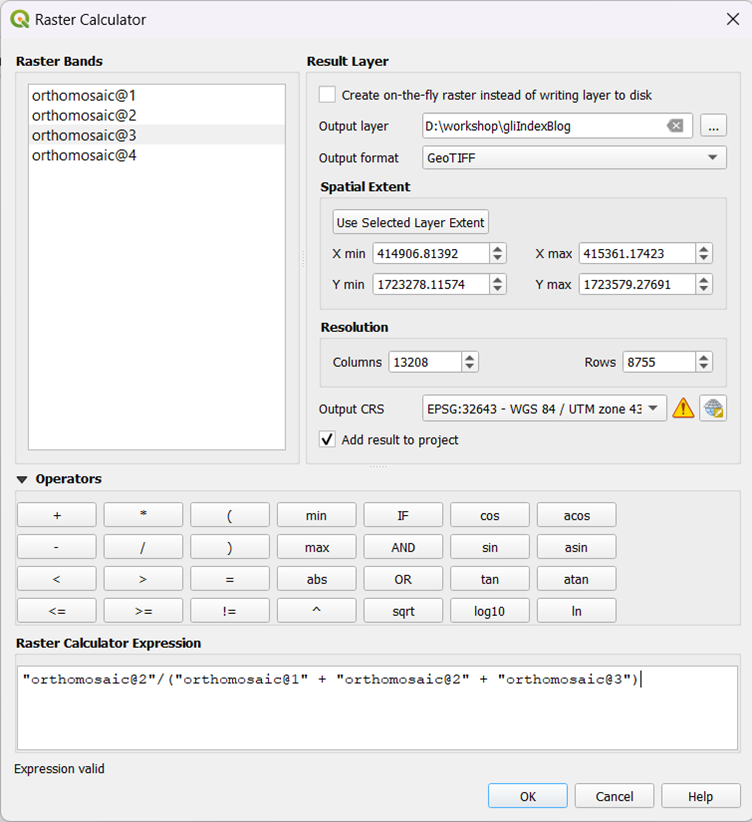
Fig. 05: Raster Calculator.
Once you have the indexed output, select appropriate symbology to view the indexed image. Right click on the layer and select ‘Properties’ or double click on the image. Navigate to Symbology option.

Fig. 06: Symbology of layer.
Select the appropriate settings for colour ramp and apply it to the indexed image.

Fig. 07: Image with selected symbology.
We see that the above image is not giving us a contrast in the image to estimate vegetation health. In this case, one can explore the blending option. This may be useful to get an immediate idea of the area at a glance.

Fig. 08: Blending options for better visual assessment.
In order to extract contrasting information from the orthomosaic and indexed image, we can check the histogram of the indexed image and then decide the minimum and maximum values based on the distribution of the image.

Fig. 09: Histogram analysis for optimising visual output.
Looking at the histogram we can tell that the range of information is encoded between 0.3 to 0.6 pixel value range. Now go back to the symbology and change the minimum and maximum values to that range.

Fig. 10: Image after rectifying minimum and maximum value range.
From the indexed image, we see that the western part of the image has lower leaf area as compared to the other parts. In order to focus on that area, create a polygon over it and draw a grid.

Fig. 11: Create a polygon layer.
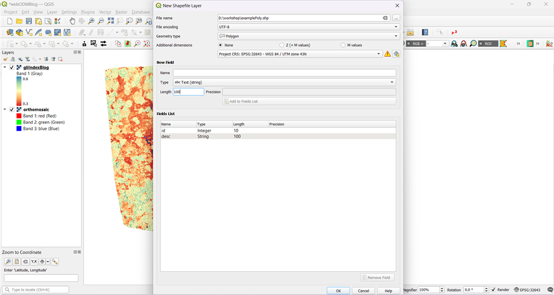
Fig. 12: Select options to create a polygon.
You must digitise a polygon in projected CRS. Projected CRS is necessary for making measurements on the shapefile.

Fig. 13: Digitise and save the polygon.
To calculate the area of the polygon, right click the polygon layer and open the attribute layer.

Fig. 14: Open attribute table.
Open the field calculator and select the option shown in the following image to calculate the area of the polygon.

Fig. 15: Select ‘area’ field from Geometry.

Fig. 16: Area field added to the polygon.
The area field is automatically calculated and added to the attribute table. It is recommended that the polygon layer has a projected CRS for this calculation to be correct. Then save edits and untoggle the editing.
You can also create a grid of squares in the polygon using the create grid tool under the vector menu.
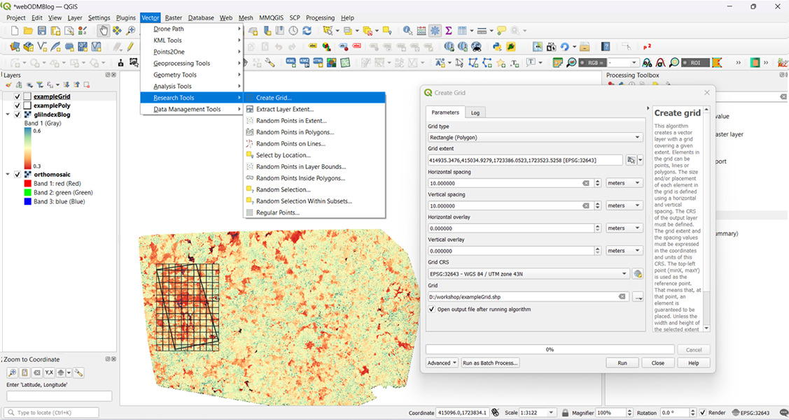
Fig 17: Creating a grid.
You can select the Rectangle type of grid, but there are other options like points, lines etc which can be chosen depending on the objective. Make sure to select the layer extent of the example polygon.
The above parameters should create a grid of rectangles of specified dimension.
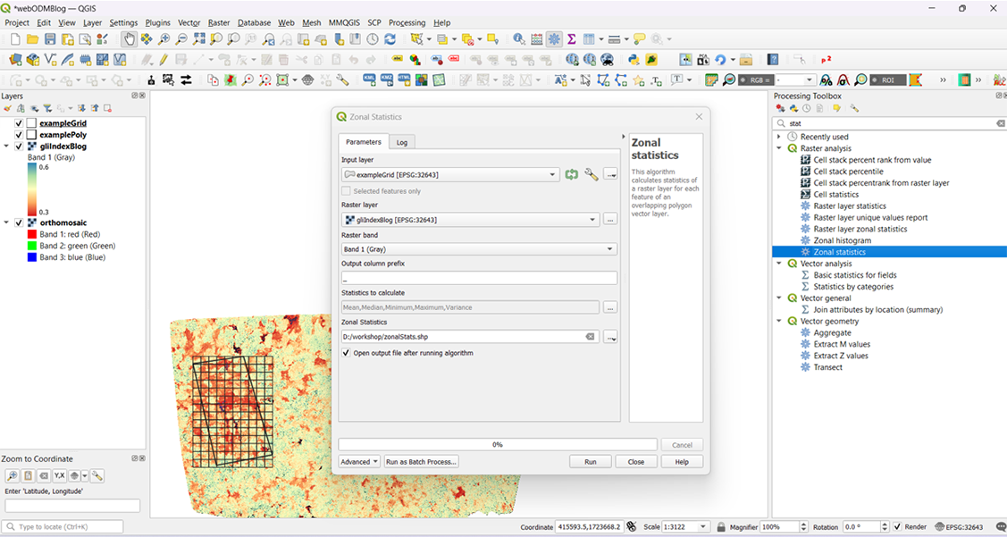
Fig. 18: Zonal statistics from Processing toolbox.
The zonal statistics can be selected from the ‘Processing toolbox’. One can select which statistics are to be calculated and a new polygon of zonal statistics will be created.

Fig. 19: Select the statistics to be calculated.
Now one can choose the statistic which they want to display and select an appropriate symbology to assess the least to most leaf cover in the selected example area as shown in the figure below.

Fig. 20: Visualise the statistical output.
In this way, we are able to analyse vegetation health of a plot from an orthomosaic created using an RGB drone.
Sources: