Assessing Ecosystem Carbon using Drones: The State of the Art

We use imagery from UAVs to calculate the heights and volume of individual mangrove trees, and can use this information to calculate the above-ground carbon stock within a given area.

While quantifying the actual value of nature may not always be possible or even desirable, the scientific community has been developing methods to quantify ecosystem services to bolster the case for the conservation of those ecosystems for a while. In our previous blogposts, we summarised methods used to estimate ecosystem carbon based on satellite imagery and field work. In this blogpost, the last in this series (for now), we examine potential methods of estimating carbon using Unmanned Aerial Vehicles (UAV). With UAVs rapidly becoming more accessible, it is important for us to understand how they could be used to provide ecosystem carbon estimates that are more accurate and precise than those derived solely from satellite data.

We examine two broad approaches to assessing carbon using UAVs. The first is based on volumetric assessments of vegetation using UAVs and the second is an attempt to use UAV-based imagery to mimic LiDAR-based methods for carbon estimation. We found several studies (Messinger, 2016; Shin, 2018; Mlambo, 2017) that demonstrated the use of UAVs for the assessment of vegetation biomass; while none of the articles we found subsequently estimated carbon, we think its possible to adapt this method for carbon estimation as well. 

A recent study by Warfield and Leon (2019) is a prime example of the first approach, of assessing vegetation volumes using UAVs. They recently conducted a comparative analysis of UAV imagery and Terrestrial Laser Scanning (TLS) to capture the forest structure and volume of three mangrove sites. The data obtained from the UAV and TLS surveys were processed to make point clouds to create 3D models from which the volume of the mangrove forest was estimated. A canopy height model (CHM) was created by subtracting a digital terrain model (DTM) from a digital surface model (DSM). This approach normalises object heights above ground, and as all the pixels in the image are linked to vegetation, the total volume is estimated by multiplying the canopy height value of a raster cell by its resolution. The UAV method produced lower height values in each patch of mangrove forest compared to the TLS surveying method and its accuracy was found to be correlated with mangrove maturity. Identifying fine scale gaps in dense forest is one of the primary limitations of using UAVs to calculate aboveground biomass. This study highlighted the suitability of utilising UAVs to calculate canopy volume in forests that are not very dense.

Though carbon stock was not calculated in the Warfield and Leon (2019) study, it can theoretically be estimated from the values obtained for the canopy volume. As shown in a report published by the USDA (Woodall, 2011), biomass can be calculated using volume, density and mass relationships, as described in equation 1.

Bodw = Vgw * SGgw * W . . . (1)

where Bodw is the oven-dry biomass (lb) of wood, Vgw is the cubic volume of green wood in the central stem, SGgw is the basic specific gravity of wood (i.e. the oven-dry mass of green volume), and W is the weight of one cubic foot of water (62.4lb).

Converting this into the metric system is a trivial calculation, and the resulting value for dry biomass can then be replaced in equation (2) to calculate carbon stock.

Cp = Bodw * CF . . . (2)

where Cp is the carbon stock within a plot, Bodw is the dry biomass in the plot and CF is the species specific carbon fraction (Goslee, 2012).

In the case of mangroves, the value for carbon fraction would be in the 0.45 to 0.48 range; in a previous blogpost, we described how Bindu et al. (2018) use a factor of 0.4759 on the AGB to generate an estimate of carbon.

The second approach for using UAVs to estimate carbon is based on a study conducted by Messinger (2016) in the Peruvian Amazon. In this study, UAVs were used to create a 3D model of the forest, which was compared with data of the same forest obtained through a LiDAR survey conducted in 2009. In order to estimate carbon stocks in the forest, the authors used a formula and coefficients developed by Asner (2013) which is a method designed to estimate regional carbon stock using LiDAR data.  For carbon estimation they used equation 3.

EACD = a * (TCH ^ b1) * ( BA ^ b2) * (R ^ b3) ………(3)

where EACD is estimated above ground carbon density, TCH is top of canopy height, BA is the regional average basal area, R is the regional average basal area-weighted wood density, and a, b1, b2, and b3 are coefficients estimated from the data.

Basal area is defined as the area within a plot that is occupied tree trunks and stems, and can be calculated using equation 4.

BA = 0.005454 * DBH^2……..(4)

We were unable to find a definite formula to calculate the regional average basal area-weighted wood density. The paper by Asner et al. (2013) uses coefficients based on fieldwork done by the authors and their team in Panama and does not specify the applicability of these coefficients to other forests. Since these coefficients are not specified as universal, it appears that one would have to conduct field work to calculate the variables for this formula. This, coupled with the ambiguity of measuring and calculating the regional average basal area-weighted wood density, makes this study difficult to replicate.

The calculation of the Top of Canopy Height also suffered a setback in this study. In order to derive the TCH, one has to first create a DTM (Digital Terrain Model) and CHM (Canopy Height Model) . The method used in this paper requires the use of LiDAR data in order to calculate canopy height.  In their study, the GPS on the drone was not accurate enough to create a good estimation of the CHM. They thus had to combine their UAV-based Structure-from-Motion model with LiDAR data to make this estimation. They state that this barrier can be overcome by the use of higher precision GPS where error in X, Y, and Z is less than 1m, which is now possible using UAVs in conjunction with directional-GPS (D-GPS) systems, such as the DJI Phantom 4 RTK.

In conclusion, we think that technology and research has advanced to a point where it can be used to carbon stocks using UAVs, but a clear methodology for doing so is still not publicly available. There is a need to synthesize existing methods into the most effective workflow based on these studies and current technology. We believe that having a clear and accessible method that has been tested for accuracy is crucial to bridge the gap between science, policy and conservation, and we’re going to be working on this over the next few months!    

References

Asner, G. & Mascaro, J. (2013). Mapping tropical forest carbon: Calibrating plot estimates to a simple LiDAR metric. Elsevier. 

Bindu,   G., Rajan,   P., Jishnu, E.   S., & Joseph, K.  A. (2018). Carbon stock   assessment of mangroves using remote sensing and geographic information system. The Egyptian Journal of Remote Sensing and Space Science.

Goslee, K., Walker, S., Grais, A., Murray, L., Casaraim, F., Brown, S. (2012). Module C-CS: Calculations for Estimating Carbon Stocks. Winrock International. 

Messinger, M., Asner, G., Silman, M. (2016). Rapid Assessments of Amazon Forest Structure and Biomass Using Small Unmanned Aerial Systems. MDPI (Remote Sensing), 8(8), 615.

Mlambo, R., Woodhouse, I., Gerard, F., Anderson, K., (2017). Structure from Motion (SfM) Photogrammetry with Drone Data: A Low Cost Method for Monitoring Greenhouse Gas Emissions from Forests in Developing Countries. MDPI (Forests), 8, 68. 

Shin, P., Sankey, T., Moore, M., & Thode, A. (2018). Estimating Forest Canopy Fuels in a Ponderosa Pine Stand. Remote Sensing, 10, 1266. 

Warfield, A., Leon, J. (2019). Estimating Mangrove Forest Volume Using Terrestrial Laser Scanning and UAV-Derived Structure-from-Motion. MDPI (Drones), 3, 32.

Woodall, C., Heath, L., Domke, G., & Nichols, M. (2011). Methods and Equations for Estimating Aboveground Volume, Biomass, and Carbon for Trees in the U.S. Forest Inventory, 2010. USDA (U.S. Forest Service).

Assessing Carbon using Satellite Imagery: the Math and Maps behind Ecosystem Valuation.

As a geospatial data consultancy with a conservation focus, we’re developing workflows that we believe will have the most conservation impact, and one of the areas we see the most promise in is in the rapid estimation of carbon stocks in a landscape. Carbon sequestration is one of the many ecosystem services intact wildlife habitat can also provide, and valuing the carbon within such ecosystems can provide an added incentive to conserve them.

In a previous blogpost, we described the process of using vegetation indices to analyse satellite and drone imagery. We’re following that up with this blogpost, where we’re going to describe how carbon stocks in a landscape can be estimated by combining satellite imagery, vegetation indices and field data.

A caveat up front: we’re using this blogpost to summarise some methods, to teach ourselves this workflow and to familiarise ourselves with the entire process. We haven’t collected our own field data for this process, and the maps themselves were made using regression coefficients extracted from the papers we’ve mentioned. The maps are a lie(!) but they’re also reasonably accurate depictions of what actual maps would look like if we had field data; they definitely do not reflect actual carbon stock values for these landscapes.

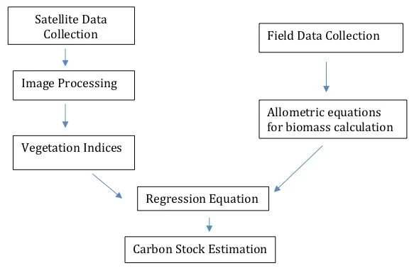
The workflow for the estimation of Above Ground Carbon

Field Data Collection

Collecting field data to estimate carbon stocks is an essential step in the process; this information is used to develop regression equations that correlate Above Ground Biomass (AGB) as observed on the ground with information obtained from satellite imagery. As collecting field data for every pixel of the image isn’t possible, a statistical sampling process is used to obtain adequate information for the entire study area, and most papers we read described using a stratified random sampling technique. In this method, plots of  the area are initially classified into classes based on specific criteria such as, for example, vegetation density. Plots from each class are then selected at random, while also accounting for other possibly related factors like species variation. Once the plots for sampling are selected, laborious field work ensues, where the biomass of individual trees within each plot is assessed. One of the most common methods to determine AGB used to be destructive sampling, where the trees randomly selected to be part of the sampling process were uprooted, and their components physically weighed. This process is expensive, labour-intensive and time consuming, and doesn’t really work when the overarching goal is the preservation of wildlife habitat. Fortunately, there’s an alternative; allometry is the science of measuring and studying the growth or size of a part in relation to an entire organism and can be used to obtain the required data non-destructively.

Allometry is a very useful way to estimate tree weight from measurements of its independent parts. However, different allometric equations have to be developed for each tree species and site which makes this process complicated. The Pipe Model Theory (Shinozaki et al. 1964a,b) showed that the above ground weight of a tree was a function of the squared diameter at trunk base and wood density. This allows for the development of common allometric equations based on species which can be applied across the geographical location of the forests. Komaya et al. (2005) for example, have developed common allometric equations for mangroves which have been used across mangroves species and areas for AGB estimation, making this process much less labour intensive and much more uniform.

Most AGB studies measure parameters such as Diameter at Breast Height (DBH) and tree height, which are then used to develop allometric equations by which the biomass of any given tree can be estimated. DBH is usually measured by wrapping a measuring tape around the primary trunk of the tree at a height of 4.5 feet (~150cm) above the ground. The height of a tree is estimated using basic trigonometry along with tools such as a laser rangefinder or a clinometer.

Carbon Stock Calculation from Vegetation Indices:

We’ve assessed some of the methods that we found in the literature and consider applicable to our work. This is not an exhaustive list and if you know of any methods that you believe are efficient or effective, please let us know! As we’ve mentioned earlier, we’ve not conducted field data collection for this blogpost and are going to be using coefficients from other papers in our calculation of carbon stock.

We acquired Landsat 8 imagery from December 2018 which was processed to obtain Top of Atmosphere (ToA) reflectance values. We analyzed these using vegetation indices as described in a previous blogpost and then used these index maps to replicate the carbon assessment workflows we found in the literature.

Bindu et al. (2008) calculated both above and below ground biomass for a mangrove forest in Kerala. They collected field data through stratified sampling and applied common allometric equations (eq 1) for mangroves developed by Komaya et al. (2005) for estimating biomass in these field sample data sets. This ground truthing is done to establish a relationship between AGB calculated from field observations and vegetation indices calculated from satellite imagery.

AGB=0.251* r * (DBH^2.46) . . . . . (1)

where ρ is species-specific wood density.

 The researchers used equation 2 developed by Myeong et al. (2006) as the relationship between Above Ground Carbon (ABC) and vegetation indices calculated from satellite imagery. They used their field data along with satellite data from Indian Space Research Organization’s LISS-IV satellite for their calculations.

AGB = a * e^(NDVI*b) . . . . . . (2)

where AGB is measured in kg per pixel, a and b are constants developed from the non-linear regression. 

In this case, a = 0.507 and b=9.933.

In mangrove forests, Below Ground Biomass (BGB) is also extremely important, and Bindu et al. (2018) found that the average ratio of BGB to AGB in their study area was 0.38. By relating AGB to BGB, they were able to estimate the total biomass and convert this into carbon values by multiplying it by 0.4759 ( which is the value this study used as the ratio of biomass to carbon).

To replicate their work, we’ve created a Normalised Difference Vegetation Index map from our Landsat 8 satellite imagery, and estimated carbon stock using their methods and regression coefficients. We’ve also converted the units from kg/pixel into tonnes/hectare to compare our results with other methods.

Estimating carbon from an NDVI map after Bindu et al. (2018), using their regression coefficients of a = 0.507 and b = 9.933.

 Laosuwan et al. (2016) studied orchards in Thailand to estimate Above-Ground Carbon directly. They used different allometric equations since they were doing this survey for agro-forestry rather than studying mangroves. For this, they collected data on height and DBH for a number of trees and combined this field data with a Difference Vegetation Index (DVI) applied on Landsat 8 imagery to create regression equations for estimating carbon stock. The exact break-down of the methodology they’ve used to develop these regression equations was not explained clearly in the paper (and we’re planning to learn more about it!) but the final equation for carbon sequestration estimated using DVI can be seen in equation 3.

ABC = a * e^(b * DVI) . . . . . (3)

where ABC is measured in tonnes/rai; one rai (a Thai unit of area) is equivalent to 0.16 hectares.

Estimating carbon from a DVI map after Laosuwan et al. (2016), using their regression coefficients of a = 0.3184 and b = 0.482.

Situmorang et al. (2016) used a completely different work flow to estimate carbon stocks. Their field data included the species name, number of trees, tree height and diameter at breast height (DBH). They used these variables to calculate biomass using the following formula derived from Chave et al. (2005).

W = 0.0509 x ρ x (DBH ^ 2) x T

where W = the total biomass (kg)

DBH = diameter at breast height

ρ = wood density (gr / cm3)

T = height (m)

This was then extrapolated to the entire area using the following formula:

After Brown et al. (1996), the carbon content is estimated to be exactly half (50%) of the biomass value.

Regression equations were then developed between two vegetation indices applied on satellite imagery, and carbon stock, in these sample areas to estimate Above Ground Carbon. Carbon stocks in the production forest of Lembah Seulawah district were calculated using the regression analysis equation y = 151.7x-39.7 on an EVI image and y= 204.3x-102.1 on a NDVI image. We attempted to use these regression equations to estimate carbon stock in our satellite image but these equations resulted in negative carbon stock values over most pixels in the satellite image we used. In fact, using the range of NDVI (0.17 - 0.85) and EVI (0.05 - 0.93) given by the researchers in their own study area, it seems possible that they would have also generated negative carbon values, which is a physical impossibility. We’re unsure if the researchers are using absolute values generated from their equation or if there are additional steps in the methodology not mentioned in the paper, but we were unable to recreate carbon stock estimates based on the methodology explained in their paper.

Some scientists have been using LiDAR (light detection and ranging) to replace field-based surveys. However, LiDAR imagery remains very expensive and is, for the most part, inaccessible. Planet, a satellite operator and provider of very high resolution satellite imagery, recently used imagery from their RapidEye and Dove satellites to estimate carbon stocks in Peru using very high resolution imagery instead of LiDAR.  Their algorithm explained 69% of the variation in their study area and they found that using spatial data with more than 5m resolution could be used for calculating biomass estimates at national level.

Our next post on this topic is going to be about developing methods where Unmanned Aerial Vehicles (UAVs) can be used to replace the ground-based field work. If you have any questions or comments, get in touch with us at contact@techforwildlife.com.

Calculating a drone camera's image footprint OR How I learned to love tan again.

When we use drones for mapping purposes, we usually program them to fly autonomously along a pre-programmed flight path, collecting images with a specified front- and side- overlap. Once we have enough images covering the area to be mapped, we stitch them all together to create the final map. This really doesn’t require us to think a lot about the length and width of each image; the only two limiting factors we usually need to consider are the final map’s (or technically, orthorectified mosaic’s) spatial resolution and the drone’s maximum legal height.

However, one of the projects we’re currently working on is not so much a mapping project as it is ecological research, and to cut a long story short, ensuring that we can correctly apply a set of ecological statistical tools that account for double-counting and observer error requires us to be able to ascertain the length and width of each image at different drone altitudes. Also, as we work with a number of different drones (and thus drone cameras), I wanted to have a set of equations in place that we could use for a variety of situations. All of this required some high-school level trigonometry to work out; I was never a fan of trigonometry as a teenager, but using it to understand both the Triangular Greenness Index (as detailed in a previous post on vegetation indices) and the current problem was actually a lot of fun.

View fullsize

View fullsize

To break the problem down, the two fixed variables are a camera’s field of view (FoV), which is described as the angle which it can ‘see’ at any given instant, and its aspect ratio, which is the ratio between the length and width of its images. For example, from the technical descriptions, a Phantom 3 Advanced camera has a FoV of 94° and user-selectable aspect ratios of 4:3 and 16:9, while the Phantom 4 Pro 2.0 has an FoV of 84° and user-selectable aspect ratios of 3:2, 4:3 and 16:9. In combination with the height of the drone, these two camera-parameters determine the final image footprint. For more on aspect ratios, see this post which recommends using the native aspect ratio for any given camera.

Caveats:

! These equations assume the camera to be perpendicular to the ground and don’t account for lens distortion. For a far more complex solution (which I have to admit I barely understand) look up this post (StackExchange) where mountainunicycler (Github user) describes nesting a Python script within Latex (what) which then calculates the FoV of a drone-mounted camera and outputs a PDF with graphics ( I can’t even.) !

---

x = Drone Height
θ = Field of View
r = Aspect Ratio

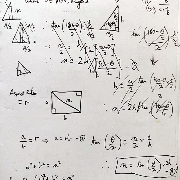
If the diagonal of the image is D, D/2 is the length of the base 
of the right-angled triangle with the two included angles as θ°/2
and (180°-θ°)/2 (as becomes clear when the FoV angle is bisected
to create two identical right-angled triangles).

D = 2 * x * tan(θ°/2)   --- (1)

If (A) and (B) are the sides of the image, then the aspect ratio 
(r) is equal to either A/B or B/A. We assume (A) to be the 
independent variable and (B) to be the dependent variable.

r = A / B
B = r * A   --- (2)

Using the equation of a right-angled triangle again,

D^2 = A^2 + B^2
D^2 = A^2 + (r * A)^2   - substituting the value of B from (2)
D^2 = A^2 * (1 + r^2)
A^2 = D^2 / (1 + r^2)       - flipping the terms of the equation

A = D / sqrt(1 + r^2)       --- (3)
B = r * D / sqrt(1 + r^2)   --- (4)

To express (A) and (B) only in terms of x, θ and r, we now 
combine equations (1) and (3), and (1) and (4).

A = (2 * x * tan(θ°/2)) / sqrt(1 + r^2) --- (5)

and

B = r * (2 * x * tan(θ°/2)) / sqrt(1 + r^2) - from (1) and (4)
B = 2 * r * x * tan(θ°/2) / (sqrt(1 + r^2) --- (6)

---

So, if we know the field of view (θ°), the aspect ratio (r) and the height of the drone (x), equations (5) and (6) allow us to determine the image footprint. To calculate the area of the image, the math is simply (A) * (B), which is the formula for the area of a triangle.

To flip this around, the other equation we needed for this project was to determine the height we needed to fly the drone, given a specific image footprint i.e. given (A), calculate (x). This is straightforward, since it means we just need to make (x) the subject, as opposed to (A), in equation (5).

---

A = (2 * x * tan(θ/2)) / sqrt(1 + r^2) --- (5)

2 * x * tan(θ/2)) = A * sqrt(1 + r^2)

x = A * sqrt(1 + r^2) / (2 * tan(θ/2)) --- (7)

---

In summary, equations (5) and (6) allow us to use the FoV, aspect ratio and height of any given camera to determine the image footprint, while equation (7) allows us to determine what height we should fly a drone at, given a desired horizontal image dimension.

I’ve used these equations to create a calculator in Excel; note that Excel uses radians as the default unit for angles. Using this calculator, I can determine that with a FoV of 94°, an aspect ratio of 4:3 and a drone height of 60m, the image footprint would be 102.9m * 77.2m, while with an FoV of 77°, an aspect ratio of 16:9 and the same drone height, the image footprint would be 83.1m * 46.8m. Similarly, if I wanted an image length of 50m with the first camera (FoV = 94° and aspect ration = 4:3), I would need to fly the drone at a height of 41.25m.

Let us know if you have any comments or find any errors in the math! We’re on Twitter at @techforwildlife, and you can mail us at contact@techforwildlife.com. As usual, comments on this post will be open for a few days.