As a geospatial data consultancy with a conservation focus, we’re developing workflows that we believe will have the most conservation impact, and one of the areas we see the most promise in is in the rapid estimation of carbon stocks in a landscape. Carbon sequestration is one of the many ecosystem services intact wildlife habitat can also provide, and valuing the carbon within such ecosystems can provide an added incentive to conserve them.
In a previous blogpost, we described the process of using vegetation indices to analyse satellite and drone imagery. We’re following that up with this blogpost, where we’re going to describe how carbon stocks in a landscape can be estimated by combining satellite imagery, vegetation indices and field data.
A caveat up front: we’re using this blogpost to summarise some methods, to teach ourselves this workflow and to familiarise ourselves with the entire process. We haven’t collected our own field data for this process, and the maps themselves were made using regression coefficients extracted from the papers we’ve mentioned. The maps are a lie(!) but they’re also reasonably accurate depictions of what actual maps would look like if we had field data; they definitely do not reflect actual carbon stock values for these landscapes.
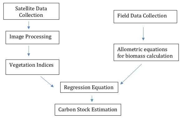
The workflow for the estimation of Above Ground Carbon
Field Data Collection
Collecting field data to estimate carbon stocks is an essential step in the process; this information is used to develop regression equations that correlate Above Ground Biomass (AGB) as observed on the ground with information obtained from satellite imagery. As collecting field data for every pixel of the image isn’t possible, a statistical sampling process is used to obtain adequate information for the entire study area, and most papers we read described using a stratified random sampling technique. In this method, plots of the area are initially classified into classes based on specific criteria such as, for example, vegetation density. Plots from each class are then selected at random, while also accounting for other possibly related factors like species variation. Once the plots for sampling are selected, laborious field work ensues, where the biomass of individual trees within each plot is assessed. One of the most common methods to determine AGB used to be destructive sampling, where the trees randomly selected to be part of the sampling process were uprooted, and their components physically weighed. This process is expensive, labour-intensive and time consuming, and doesn’t really work when the overarching goal is the preservation of wildlife habitat. Fortunately, there’s an alternative; allometry is the science of measuring and studying the growth or size of a part in relation to an entire organism and can be used to obtain the required data non-destructively.
Allometry is a very useful way to estimate tree weight from measurements of its independent parts. However, different allometric equations have to be developed for each tree species and site which makes this process complicated. The Pipe Model Theory (Shinozaki et al. 1964a,b) showed that the above ground weight of a tree was a function of the squared diameter at trunk base and wood density. This allows for the development of common allometric equations based on species which can be applied across the geographical location of the forests. Komaya et al. (2005) for example, have developed common allometric equations for mangroves which have been used across mangroves species and areas for AGB estimation, making this process much less labour intensive and much more uniform.
Most AGB studies measure parameters such as Diameter at Breast Height (DBH) and tree height, which are then used to develop allometric equations by which the biomass of any given tree can be estimated. DBH is usually measured by wrapping a measuring tape around the primary trunk of the tree at a height of 4.5 feet (~150cm) above the ground. The height of a tree is estimated using basic trigonometry along with tools such as a laser rangefinder or a clinometer.
Carbon Stock Calculation from Vegetation Indices:
We’ve assessed some of the methods that we found in the literature and consider applicable to our work. This is not an exhaustive list and if you know of any methods that you believe are efficient or effective, please let us know! As we’ve mentioned earlier, we’ve not conducted field data collection for this blogpost and are going to be using coefficients from other papers in our calculation of carbon stock.
We acquired Landsat 8 imagery from December 2018 which was processed to obtain Top of Atmosphere (ToA) reflectance values. We analyzed these using vegetation indices as described in a previous blogpost and then used these index maps to replicate the carbon assessment workflows we found in the literature.
Bindu et al. (2008) calculated both above and below ground biomass for a mangrove forest in Kerala. They collected field data through stratified sampling and applied common allometric equations (eq 1) for mangroves developed by Komaya et al. (2005) for estimating biomass in these field sample data sets. This ground truthing is done to establish a relationship between AGB calculated from field observations and vegetation indices calculated from satellite imagery.
AGB=0.251* r * (DBH^2.46) . . . . . (1)where ρ is species-specific wood density.The researchers used equation 2 developed by Myeong et al. (2006) as the relationship between Above Ground Carbon (ABC) and vegetation indices calculated from satellite imagery. They used their field data along with satellite data from Indian Space Research Organization’s LISS-IV satellite for their calculations.
AGB = a * e^(NDVI*b) . . . . . . (2)where AGB is measured in kg per pixel, a and b are constants developed from the non-linear regression. In this case, a = 0.507 and b=9.933.In mangrove forests, Below Ground Biomass (BGB) is also extremely important, and Bindu et al. (2018) found that the average ratio of BGB to AGB in their study area was 0.38. By relating AGB to BGB, they were able to estimate the total biomass and convert this into carbon values by multiplying it by 0.4759 ( which is the value this study used as the ratio of biomass to carbon).
To replicate their work, we’ve created a Normalised Difference Vegetation Index map from our Landsat 8 satellite imagery, and estimated carbon stock using their methods and regression coefficients. We’ve also converted the units from kg/pixel into tonnes/hectare to compare our results with other methods.

Estimating carbon from an NDVI map after Bindu et al. (2018), using their regression coefficients of a = 0.507 and b = 9.933.
Laosuwan et al. (2016) studied orchards in Thailand to estimate Above-Ground Carbon directly. They used different allometric equations since they were doing this survey for agro-forestry rather than studying mangroves. For this, they collected data on height and DBH for a number of trees and combined this field data with a Difference Vegetation Index (DVI) applied on Landsat 8 imagery to create regression equations for estimating carbon stock. The exact break-down of the methodology they’ve used to develop these regression equations was not explained clearly in the paper (and we’re planning to learn more about it!) but the final equation for carbon sequestration estimated using DVI can be seen in equation 3.
ABC = a * e^(b * DVI) . . . . . (3)where ABC is measured in tonnes/rai; one rai (a Thai unit of area) is equivalent to 0.16 hectares.

Estimating carbon from a DVI map after Laosuwan et al. (2016), using their regression coefficients of a = 0.3184 and b = 0.482.
Situmorang et al. (2016) used a completely different work flow to estimate carbon stocks. Their field data included the species name, number of trees, tree height and diameter at breast height (DBH). They used these variables to calculate biomass using the following formula derived from Chave et al. (2005).
W = 0.0509 x ρ x (DBH ^ 2) x Twhere W = the total biomass (kg)DBH = diameter at breast heightρ = wood density (gr / cm3)T = height (m)This was then extrapolated to the entire area using the following formula:

After Brown et al. (1996), the carbon content is estimated to be exactly half (50%) of the biomass value.
Regression equations were then developed between two vegetation indices applied on satellite imagery, and carbon stock, in these sample areas to estimate Above Ground Carbon. Carbon stocks in the production forest of Lembah Seulawah district were calculated using the regression analysis equation y = 151.7x-39.7 on an EVI image and y= 204.3x-102.1 on a NDVI image. We attempted to use these regression equations to estimate carbon stock in our satellite image but these equations resulted in negative carbon stock values over most pixels in the satellite image we used. In fact, using the range of NDVI (0.17 - 0.85) and EVI (0.05 - 0.93) given by the researchers in their own study area, it seems possible that they would have also generated negative carbon values, which is a physical impossibility. We’re unsure if the researchers are using absolute values generated from their equation or if there are additional steps in the methodology not mentioned in the paper, but we were unable to recreate carbon stock estimates based on the methodology explained in their paper.
Some scientists have been using LiDAR (light detection and ranging) to replace field-based surveys. However, LiDAR imagery remains very expensive and is, for the most part, inaccessible. Planet, a satellite operator and provider of very high resolution satellite imagery, recently used imagery from their RapidEye and Dove satellites to estimate carbon stocks in Peru using very high resolution imagery instead of LiDAR. Their algorithm explained 69% of the variation in their study area and they found that using spatial data with more than 5m resolution could be used for calculating biomass estimates at national level.
Our next post on this topic is going to be about developing methods where Unmanned Aerial Vehicles (UAVs) can be used to replace the ground-based field work. If you have any questions or comments, get in touch with us at contact@techforwildlife.com.